Solving classification problems by Liquid State Machines (LSM) usually ignores the influence of the liquid state representation on performance, leaving the role to the reader circuit. In most studies, the decoding of the internally generated neural states is performed on spike rate-based vector representations. This approach occults the interspike timing, a central aspect of biological neural coding, with potentially detrimental consequences on the LSM performance. In this work, we propose a model of liquid state representation that builds the feature vectors from temporal information extracted from the spike trains, hence using spike synchrony instead of rate. Using pairs of Poisson-distributed spike trains in noisy conditions, we show that such model outperforms a rate-only model in distinguishing two spike trains regardless of the sampling frequency of the liquid states or the noise level. In the same vein, we suggest a synchrony-based measure of the separation property (SP), a core feature of LSMs regarding classification performance, for a more robust and biologically plausible interpretation.

1. Introduction

Liquid State Machines (LSMs) are generic models of computation inspired by biological cortical circuits. As such, they are well suited for real-time, online and anytime computations, and they can under certain circumstances exhibit unlimited computational power [1].  One important aspect of LSMs is their conceptual simplicity and relative ease of implementation in comparison to multilayer networks with error backpropagation training. LSMs have been tested with relative success in a variety of experimental contexts: identification of spoken words, voice, phonemes [2], [3], [4] and musical instruments [5], [6], robotics [7], movement prediction [8]; classification of musical styles [9], seismic data for military vehicles [10], nuclear stockpile data [3]; recognition of signature counterfeits  [11], and even the study of biological neurons [12]. However, the LSM performance for classification tasks is variable [13], [14], [15], [16], potentially due to the randomly connected and untrained liquid regardless of application. Several authors have investigated liquid optimization approaches to raise the performance of LSMs, including Genetic Algorithms [13], [17], Separation Driven Synaptic Modification [18], Reinforcement Learning [17], Particle Swarm Optimization [19], and a number of different learning methods for temporal representations of artificial spiking neural networks (statistics, Hebbian learning, gradient estimation, linear algebra formalisms, etc.) that are reviewed in [20].  

Still, the research on LSMs rarely focuses on the influence of the liquid state representations on performance. In most studies, the decoding of the discrete input spike trains relies on rate-based feature vectors used as inputs to a classifier. The rate coding typically counts the number of spikes in arbitrary time bins and filters the results with an exponential kernel due to its shape resemblance to the postsynaptic currents in biological neurons [21]. This ignores the spike timing, with potentially detrimental consequences on LSM classification performance. In this work, we propose a model of the liquid states that is based on temporal information extracted from the input spike trains, aiming to improve classification performance without increasing the liquid’s dimensionality. We show that this model outperforms a rate-based model at classifying Poisson-distributed spike trains in noisy conditions regardless of the sampling frequency of the liquid states. We therefore suggest a synchrony-based measure of the Separation Property (SP) of LSMs, for a more robust and biologically plausible interpretation.

This paper is divided as follows: the next section provides a brief description of the LSM model, with examples of use in classification problems. In section III, we focus on the common rate-based representation of liquid states to show that it leaves apart critical temporal information about spike trains. We also review the known measures of SP and underline the absence of synchrony-based methods to quantify it. Section IV proposes a novel representation of the liquid state based on spike metrics, as well as a composite state model that incorporates both rate and temporal representations in a composite feature vector. We also describe the methodology used to test performance hypotheses about synchrony in the context of classifying Poisson-distributed input spike trains, as well as the correlation of performance with SP measures. We present the simulation results in Section V before a discussion and conclusions.

2. The Liquid State Machine Model (LSM)

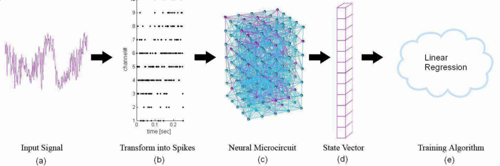
Figure 1 summarizes the processing steps in the LSM model, showing the input signal encoding (a, b), the spatio-temporal propagation within the liquid (c), the liquid state vector coding (d) and the interpretation by a readout mechanism (e).  The core of the LSM is the neural liquid, or microcircuit, which consists in a grid of interconnected artificial spiking neurons, usually in 3-dimensional space by analogy to biological cortical columns (see Figure 1.c). The neurons occupy the nodes of this structure and are usually connected by randomly generated synapses. Due to its inputs and recurrent connections, the liquid forms a dynamic system endowed with the memory of previous states [4], [22], [23]. As a result, it continuously projects input signals onto a high-dimensional space. This mapping fosters the emergence of spatiotemporal patterns (trajectories, or “time-varying changes in the active state” [24], p. 114) that may be identified by simple, memoryless readouts [13], [3], as long as two major constraints are enforced: the Approximation Property (AP) and the Separation Properties (SP); AP guarantees that the readout can approximate any function of the liquid states to an arbitrary level of accuracy, whereas SP ensures that trajectories produced in the liquid by different input stimuli are well differentiated.

The readout maps liquid states to meaningful outputs; in the case of classification, it projects state vectors onto classes. Similar to Support Vector Machines, the capability to separate complex trajectories by linear discriminators is guaranteed by the fact that the “the dimension of the state space exceeds the ‘complexity’ of the trajectories” [24].

The readout is the only LSM element that requires training, which may confer an advantage to the model over alternative architectures, since training a recurrent network of artificial spiking neurons can be a hard problem. However, the way the liquid states are encoded to serve as input feature vectors to the readout may play a role in achieving peak performance. This subject seems to have been largely ignored by the research community and most studies represent the liquid states by the same approach: measuring the spike rate in preset time intervals. Therefore, any potential phase information benefit is lost.

2.1. Models of Liquid States

Two broad approaches to represent the liquid states can be seen in the literature: sampling of analog signals [25], [10], such as the postsynaptic potential or the neural membrane voltage [26] and spike train decoding [23], [27], [28], [29], [8], [24]. T the typical representation in the latter is a state matrix obtained by filtering the discrete spike trains generated within the liquid after exposure to a stimulus ([3], [13], [30], [27], [10]). The filtering step is typically performed by convolution with an exponential kernel due to its resemblance to the shape of postsynaptic currents [21]. As a result, the spike firings within a liquid composed of N neurons are converted into an N-dimensional continuous signal [24], and each element of the state matrix stores the sampled values of this signal for a given observation interval, sampling rate, and neuron in the liquid. This representation is in effect a “rate code” (whereas small bin sizes can turn the representation into a “coincidence detector” [21]).

Although widely used to represent the liquid states, rate-based feature vectors miss a key aspect of the neural code: the actual timing of spike emissions, hence neglecting phase information [20], [31], [32]. On the other hand, it is now accepted that neural coding cannot be fully understood by only examining the rate of spike firing [33], [18], [34], [35], [36], [32], [31], and that the spike timing also encodes information. Hence, the synchrony between spike trains may be a cornerstone for understanding neural codes, as “temporal codes employ those features of the spiking activity that cannot be described by the firing rate.” [32]

The temporal decoding of liquid states has already been suggested before. In [29], the authors underline the potential power of the temporal relationships between the spike trains in the liquid, while [3] advocates the use of readouts that incorporate spike timings, but no study has examined the respective efficiency of synchrony-based and rate-based approaches. Similarly, SP models that consider the synchrony between spike trains in the liquid are rare [18].

2.2. Separation Property

The Separation Property evaluates the amount of “separation between the trajectories of internal states” [23] that are triggered in the liquid by two different input stimuli. The more separation, the easier it is for a readout endowed with the approximation property to distinguish between two different state trajectories in the liquid. This macroscopic property of the liquid can thus contribute to LSM classification performance.

While SP is widely regarded as a crucial predictor of performance, there is little consensus on how to measure it. The literature reveals different views, including statistical methods [13], [3], [37], and linear algebra formalisms [14] or vector distances between filtered firing rates [23], [1], [37]. For instance, Maass [23], [1] expresses SP as the Euclidean distance between the filtered state vectors of each neuron (Gaussian kernel), Dockendorf [37] uses both the Van Rossum [38] metric – which exploits the notion of distance between filtered states – and a custom measure based on the cross-correlation of spike times, Legenstein and Maass [14] link SP to the number of linearly independent variables in the state matrix, suggesting that the rank of the matrix is a good measure of separation, and Goodman and Ventura [3] and Hourdakis and Trahanias [13] use statistical methods to measure SP, with the former relying on centroids and the latter on Fisher’s Discriminant Ratio (FDR). In the following section, we describe our synchrony matrix-based approach to liquid state representation, the methodology used to investigate the ensuing effect on classification performance, and we underline the relationship between the Separation property and LSM performance.

3. Classification with temporal liquid state representations

The proposed liquid state representation is based on the synchrony level between spike trains during a given time window, as quantified by metrics that evaluate the temporal similarity between the spike trains emitted by neuron pairs in the liquid. Thus, the metrics operate on spike timings rather than counts and, as stated in [39], p. 146, “If a spike metric leads to a high-fidelity representation, then the temporal features that it captures are candidates for neural codes.”

3.1. Synchrony matrix representation of liquid states

The synchrony matrix is constructed thanks to the Adaptive Spike Distance (ADS) metric ([40], [41], [42], [43], [44], [45]), although any other bivariate spike metric may be employed. We chose ADS for its sensitivity to spikes coincidence and the fact that it does not rely on a time-scale parameter.

Given two spike trains #1 and #2 of duration T, ADS is calculated by averaging their instantaneous “dissimilarity profiles”, which measure how coincident the two spike trains are at any point in time. We have:

$$Ds = \frac{1}{T} \int_{t=0}^{T} S(t)\, dt \tag{1}$$

where Ds quantifies the overall dissimilarity between the two spike trains over T, and S(t) provides a joint measure of their instantaneous dissimilarity profiles at each time t. S(t) is defined by:

$$S(t) = \frac{S_1(t) x_{ISI}^{(2)}(t) + S_2(t) x_{ISI}^{(1)}(t)}{2 \langle x_{ISI}^{(n)}(t) \rangle^2_n} \tag{2}$$

where x⁽ⁱ⁾_isi(t) stands for the instantaneous interspike interval of spike train #i,  is the mean interspike interval for both spike trains, and S₁(t) and S₂(t) are given by:

$$S_i(t) = \frac{\Delta t_P^{(i)}(t) x_F^{(i)}(t) + \Delta t_F^{(i)}(t) x_P^{(i)}(t)}{x_{ISI}^{(i)}(t)}, \quad i = 1, 2 \tag{3}$$

In the previous equation, for spike train #i, x⁽ⁱ⁾_P(t) and x⁽ⁱ⁾_F(t) are the time latency to the closest previous spike and closest following spike at time t, respectively, and Δt_P⁽ⁱ⁾ and Δt_F⁽ⁱ⁾ are the same latency from one of these spikes to the nearest one in the other spike train. For example, Δt_P⁽¹⁾ is defined as:

$$\Delta t_P^{(1)}(t) = \min \left( \left| t_P^{(1)}(t) – t_i^{(2)} \right| \right) \tag{4}$$

where  is the time of occurrence of the closest previous spike in spike train #1 at time t, and  is the time of occurrence of the ith spike in spike train #2. A more comprehensive description of ADS with graphical illustrations can be found in [46]. Table 1 provides the example of a synchrony matrix for a liquid made of 4 neurons, where d(a, b) evaluates the dissimilarity between the spike trains of neurons a and b as with equation (1).

Given the symmetry of the synchrony matrix and its zero diagonal, the final representation may consist only in the lower triangular matrix expressed as a vector. For a liquid composed of N neurons, the size E of this vector is:

$$E = \sum_{n=1}^{N} n = \frac{(1 + N)N}{2} – N \tag{5}$$

3.2. Composite-state vector

 Theoretically, rate and synchrony represent complementary information, since they encode two aspects of the spiking within a liquid (see [39], p.148, for an in vivo example). Therefore, taking inspiration from [10], we can enhance the representation of liquid states by combining filtered rates and synchrony information. Then, the size of the features vector extracted from the liquid would increase by N. For example, N=8 would lead to a vector of 8 rate elements (one for each neuron) and 28 synchrony elements (from equation 5). We expect this composite state representation to lead to better classification results than by only using rate-based or synchrony-based representations.

A.   SP quantification with spike metrics

Using the hypothesis that the spike trains generated for different classes of input signals are significantly dissimilar (i.e., distant or unsynchronized), SP expresses the average spike train dissimilarities in the liquid. To build this synthetic measure out of spike distance metrics, we proceed similarly to getting the Fisher’s discriminant ratio (FDR) of a 2-class classification problem:

1) For each stimulus belonging to one of the classes, we build the list of corresponding liquid states, composed of the spike trains of each neuron in the liquid for the duration of the experiment.

2) we then sample pairs of liquid states by including one from one class and one from the other.

3) we measure the dissimilarity for each sampled pair with a distance metric. The separation measure is the mean of the obtained results.

 In this paper, we test cost-based measures (Victor-Purpura distance [47], [48], vector embedding (Van Rossum distance [38], Schreiber Similarity [49], Hunter-Milton Reliability [50]), scale-free measures (Spike Synchronization, ISI Distance, Spike Distance [51], [52], [40], [41], [42], [43], [44], [45] and statistical methods (Jolivet Coincidence [53]. The methodology for verifying the efficiency of these new approaches in described next.

4. Methodology of Testing

To test the performance of each model, we aggregate and compare the error rates of randomly generated LSMs at classifying Poisson-distributed spike trains, using rate-based, synchrony-based and composite liquid state representations. As a corollary, we also quantify how the synchrony-based SP measures correlate with the error rate.

4.1. Experimental setup

Three hundred random liquids are generated and fed with as many jittered versions of two template spike trains. These input signals are generated by adding temporal noise (“jitter”) to each template. Hence, each spike of the template is randomly shifted in time by an amount drawn from a uniform distribution with mean 0 and standard deviation equal to the desired jitter level. The values used in this paper

Table 2: Classification experiments and corresponding spike train templates
Experiment	First spike train before and after filtering	Second spike train before and after filtering
1: Two high-frequency spike trains ( ƛ1= ƛ2=100)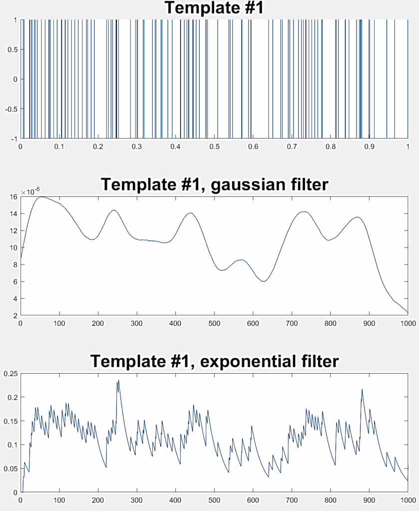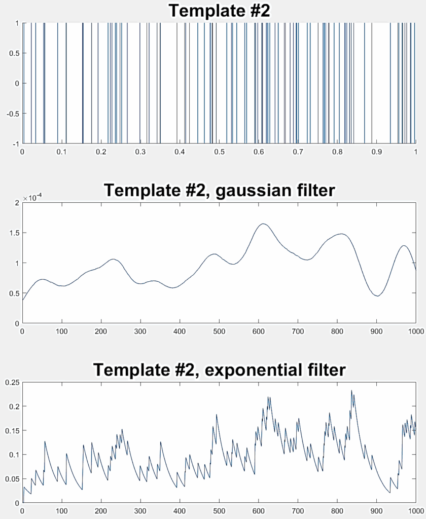
2: Two low-frequency spike trains ( ƛ1= ƛ2=20)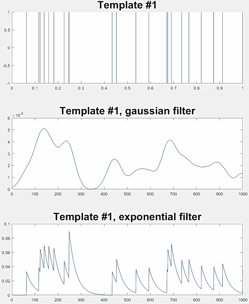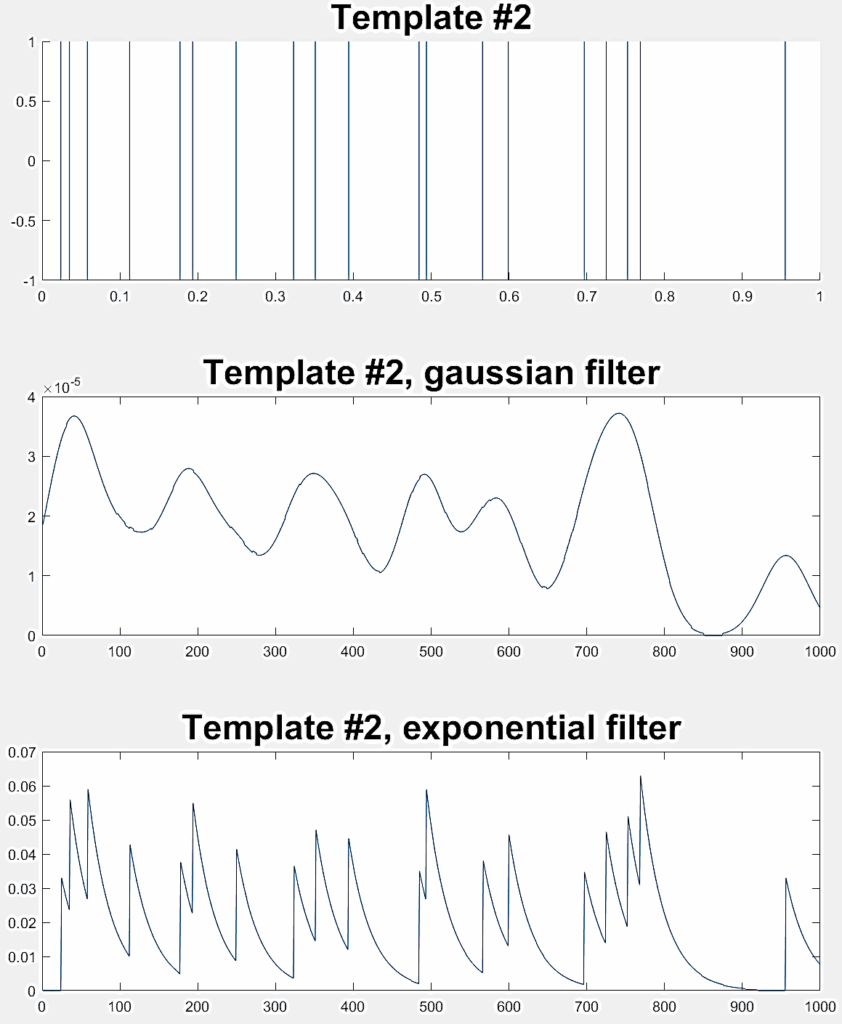
3: One high-frequency spike train (ƛ1=  100) and one low-frequency  spike train (ƛ2=20)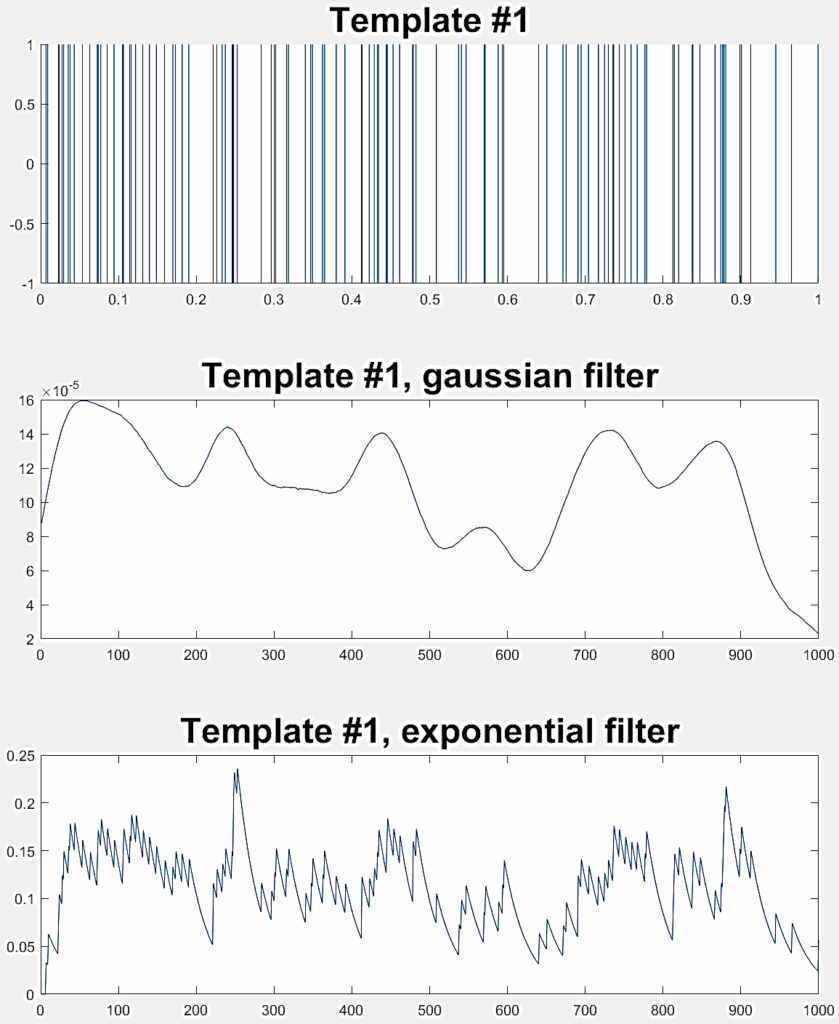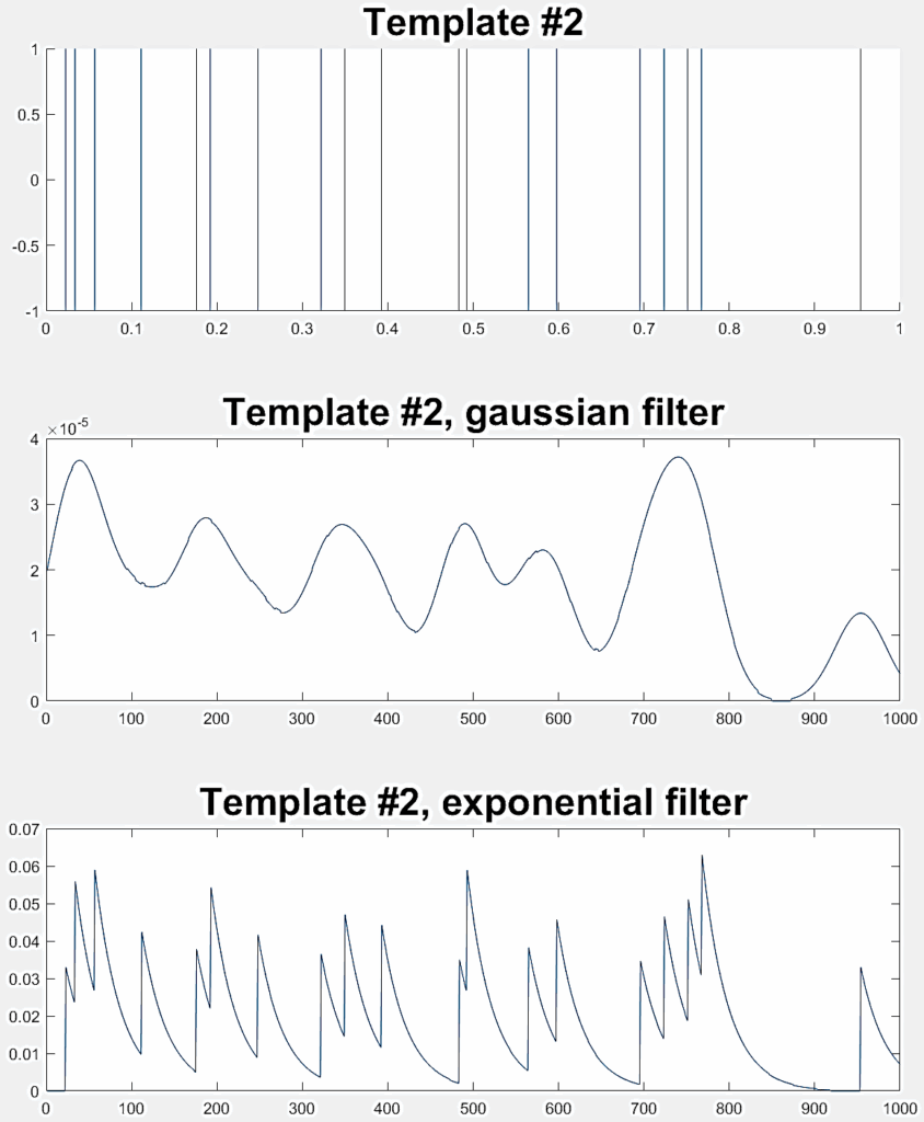

(1 ms, 4 ms, 10 ms) are loosely inspired by [23] who used 4 ms and 8 ms in their “high jitter” experimental contexts.

the original spike train pair, of which 200 are used to train the readout and 100 to collect the testing error.

The spike output from the LSM is recorded, sampled, and processed in three different ways to represent the liquid states:

1. Sampling and exponential filtering by convolving the spike trains with an exponential kernel of width 0.3 (rate coding);
2. Sampling and calculating the synchrony matrix (synchrony coding);

Aggregating the two previous representations into a composite one (composite coding).

Three different experiments are conducted to evaluate the LSM classification performance, each one involving a pair of random Poisson distributed spike trains. Table 2 indicates the ƛ value of each train (taken from [40]) with example realizations before and after filtering for rate coding. Each experiment considers 300 jittered variations of

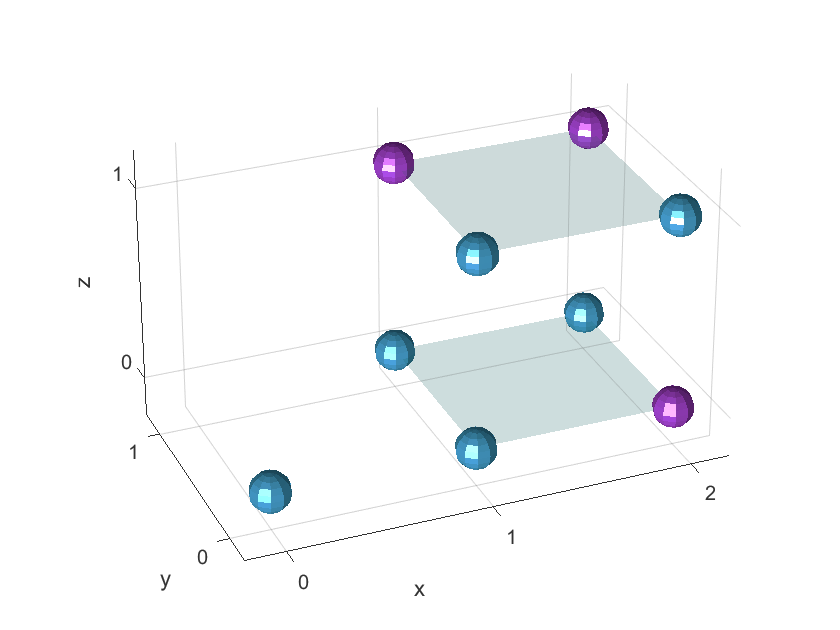
4.2. Neural Microcircuit

The liquid is organized as a 2x2x2 column (two layers of 2×2 neural grids), composed of 80% excitatory and 20% inhibitory Leaky Integrate and Fire (LIF) neurons as in [54], with dynamic synapses. A single input neuron connects to the liquid pool, and static synapses are set randomly based on the physical distance between pairs of neurons. The probability of establishing a connection is as follows [30]:

$$p = C e^{- \left( \frac{D(a,b)}{\lambda} \right)^2} \tag{6}$$

where λ is a connection parameter that controls both the average number of connections and the average distance between connected neurons [45], D(a, b) is the Euclidean distance between two neurons a and b, and C is a scaling parameter influenced by the excitatory or inhibitory effect of the connected neurons. In this study, λ was set to 2 so that any pair of neurons in the liquid column might be connected, and C was set to different values taken from previous studies ([23], [30]) and based on measures taken from cortical brain areas [30]. By default, they are set at 0.3 (for a connection between a pair of Excitatory-Excitatory neurons), 0.2 (Excitatory-Inhibitory), 0.4 (Inhibitory-Excitatory), and 0.1 (Inhibitory-Inhibitory). All other parameters are left untouched.

The chosen dimensions for the liquid allow for a large range of performance levels throughout the tests, depending only on the neuron type and connection topology of the liquids. We can easily generate drastically different liquid configurations, which in turn endow each LSM with largely different performance levels. An example of a 2x2x2 microcircuit is presented in Figure 2, where the neurons shown in cyan are excitatory, and those in magenta are inhibitory. The input neuron is the one located at position (0,0,0).

The neural dynamics are set by the following membrane voltage equation (from [55] and [56]):

$$\tau_m \frac{d v_m}{dt} = – (V_m – V_{\text{resting}}) + R_m \left( I_{\text{syn}}(t) + I_{\text{inject}} + I_{\text{noise}} \right) \tag{7}$$

where τ_m represents the membrane time constant, V_m the membrane potential, V_resting the resting membrane potential, R_m the input resistance, I_syn the current supplied by the synapses (also called “post-synaptic current” or PSC), I_inject an optional background current and I_noise is a Gaussian random variable with mean 0 and a given variance. At time t = 0, V_m is set to a default voltage V_init. During the course of the simulation, a spike is emitted if V_m exceeds a threshold V_thresh: the membrane potential is then reset to a given voltage V_reset and remains at this level for the duration of the absolute refractory period T_refract. Table 3 summarizes the values of these parameters during simulations. They are the default values of the simulation tool (see simulation tool subsection below).

The amplitude of the postsynaptic current (I_syn) depends on previous spike activity, which constitutes a form of short- term plasticity (the model is described in [57]). The total post-synaptic current going into a neuron j from all the neurons i connected to it after a spike is described by the following equation:

$$I_{\text{syn}}(t) = \sum_i I_{ij}(t) \tag{8}$$

where

$$I_{ij}(t) = w_{ij} \cdot \exp\left( \frac{-t}{\tau_{\text{syn}}} \right) \tag{9}$$

and I_ij(t) is the post-synaptic current flowing from neuron i and j; w_ij is the synaptic strength of the connection, and  is the synaptic time constant.

Contrary to static synapses, w_ij varies with previous spike trains for dynamic synapses as follows [57]:

$$w_{ij} = W \cdot r_n \cdot u_n \tag{10}$$

where W is the absolute synaptic efficiency (or weight); r_n and u_n quantify the short-term depressing and facilitating effects after spike n has been fired. The two variables are described by the following two equations [57]:

$$r_{n+1} = r_n (1 – u_{n+1}) \cdot \exp\left( \frac{-\delta t}{\tau_{\text{rec}}} \right) + 1 – \exp\left( \frac{-\delta t}{\tau_{\text{rec}}} \right) \tag{11}$$

and

$$u_{n+1} = u_n \cdot \exp\left( \frac{-\delta t}{\tau_{\text{facil}}} \right) + U \left( 1 – u_n \cdot \exp\left( \frac{-\delta t}{\tau_{\text{facil}}} \right) \right) \tag{12}$$

As indicated in [45], the absolute synaptic weights for a given connection are drawn from a gamma distribution with mean W and standard deviation .  is the elapsed time between spike n and n+1;  and  are the time constants of the facilitating and depressing plasticity effects respectively. U is a constant describing the fraction of the absolute synaptic efficiency used. The values of these parameters are indicated in Table 4.

2. Sampling, memory and decoding liquid states – The liquid states must be sampled in time in order to construct the input state vectors to the readout, with the sampling time window having an impact on classification performance. Although LSMs are known to possess “the capability to hold and integrate information from past input segments over several hundred ms” ([40], p.8), shorter sampling intervals typically provide less spike information. The scarcity of spike information in these samples can make classification harder, for an increased classification error rate. Thus, the memory span capability of LSMs plays a crucial role in providing liquid state samples with information from the past, effectively enriching them through the temporal integration of input stimuli: any state of the liquid will then keep some memory of previous states, which allows the readout to be memoryless.

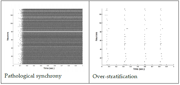
The role of memory in the classification performance of LSMs is relatively under-studied, but two extreme spike train patterns can emerge from pathological liquids: over-stratification ([15], [3]) and pathological synchrony [15]. The former happens when spikes are not propagated for a long enough time, resulting in a lack of memory capacity; the latter is the result of infinite feedback loops within the neurons, effectively spiking in synchrony and obfuscating the “real”, important states. Figure 3 shows an example of each case.

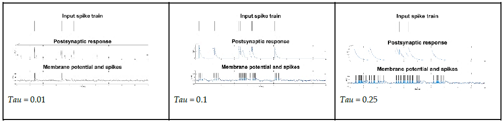
Another important parameter to consider is Tau, the synaptic time constant controlling the time required for the postsynaptic response to fade to zero after being injected with current. Figure 4 illustrates the examples of an input spike train, the postsynaptic response and the resulting spike train for three different values of Tau.

In this work, Tau is set to 0.25, a value that increases the overall performance across all tests and all liquid state representations while avoiding temporal stratification and pathological synchrony.  The choice of sampling rates (10 Hz, 4 Hz and 2 Hz) was inspired by similar values used in the literature [3], [2], [8], [29], [10].

4.3. Readout

A simple linear regression was chosen to avoid the potential impact of more advanced techniques such as multi-layer perceptrons, Support Vector Machines, etc., which may provide hard to interpret results due to their own capabilities. Thus, the predicted class value _i  of a feature state vector  is given by:

$$\hat{y}_i = m \cdot x_i + b \tag{13}$$

where m, the slope of the separating hyperplane and b, the intercept, are estimated using the least squares method. The output of this simple readout is passed through a step function for binary classification: for a given value n returned by the regression, the class y[n] is given by the following equation:

$$y[n] = \begin{cases} -1, & n \leq 0 \\ 1, & n > 0 \end{cases} \tag{14}$$

4.4. Simulation tool

We use CSIM (Circuit SIMulator, [58]), a neural network simulator that can handle LSM models with different neuron and synapse models. CSIM is built in C++ for performance considerations and provides an easy-to-use MATLAB interface. This tool uses the exponential Euler method of numerical integration, with a default time step for the update of 0.1 ms. A thorough description and a comparison to other simulators are provided in [55] and [59]. Each stimulus is simulated for 1000ms, and we used the default parameter values indicated in Table 3 for the neural dynamics (equation 7) and in Table 4 for the synaptic dynamics (equations 8 to 12)

4.5. Aggregate measure of error

The classification error of each simulation is measured as the MAE (Mean Average Error) of the training and testing steps (only the testing results are presented herein). The aggregate error for all 300 LSMs is the median of the individual errors. We chose the median over the mean because it mitigates outlier effects due to the large variations of performance observed in different LSMs, thus providing a “truer” portrait of performance. These measures are compared for equality at a 99% confidence level by a Wilcoxon rank-sum test for medians (the mean MAEs are also recorded and tested for equality using a t-Test for validation purposes). The results obtained for the “filtered rates” representation serve as a baseline for the other tests.

In all, 27 experiments are performed, each with a unique combination of the following parameters:

• 3 sample rates (10 Hz, 4 Hz, 2 Hz);
• 3 levels of jitter (1 ms, 4 ms, 10 ms);
• 3 stimuli pairs frequency patterns (100-100 Hz, 20-20 Hz and 100-20 Hz).

5. Results

We begin with the efficiency of the temporal coding of liquid states and the roles of sampling rate, jitter and memory capabilities. Then, we consider the problem of larger liquids and finally present the results on the new models of SP.

5.1. Filtered rates vs. Synchrony matrix vs. composite representations.

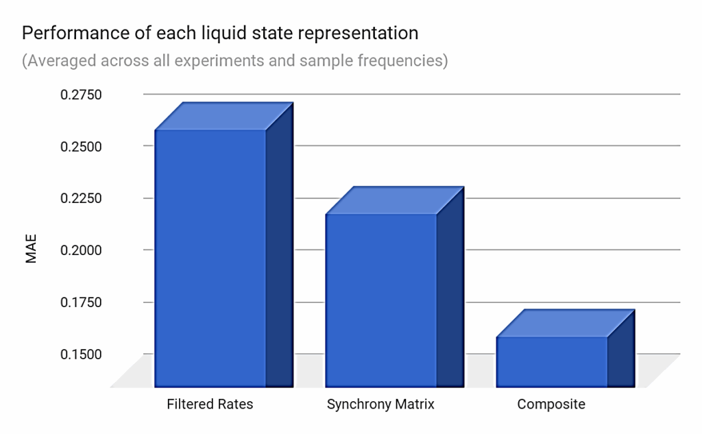
Figure 5 reports the MAE results for the three types of liquid state representations averaged across all 27 experiments and sample frequencies. It shows a significantly better performance of the composite-state approach over the other state representations (36% better than using filtered rates).

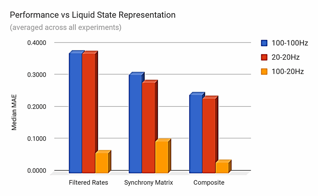
The synchrony-matrix state representations ranked second behind the composite-state approach on average, but the synchrony-only representations performed slightly worse than the rate-based ones when the stimuli pairs were of different spike emission rates (i.e., 100 Hz and 20 Hz). In this case, the difference between the rates of emission led to clearly distinct rate-based representations, resulting in better performance as seen in Figure 6.

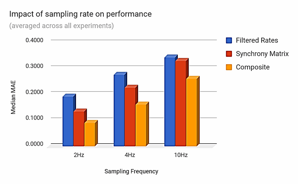
5.2. Impact of the sampling frequency

Figure 7 shows that higher sampling rates degrade the classification performance. This can be explained by the fact that less information is then conveyed by each sample, albeit temporal resolution is increased.

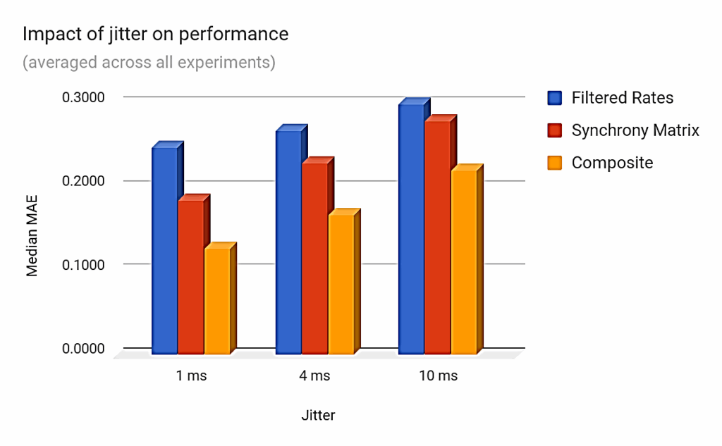
5.3. Impact of jitter on performance

Here also, increased levels of temporal noise decrease performance as may be expected. The degradation is significant as shown in Figure 8, but it appears to be less important than when using different sampling frequencies. Even a 10 ms jitter (representing between 10% and 50% of the stimulus base frequency) has a limited effect on classification error.

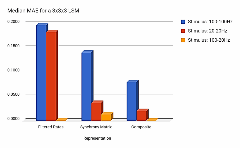
A.   Effect of a bigger cortical column

The previous observations remain valid for a 3x3x3 LSM. Figure 9 shows the relative performance of each liquid state representation and for each of the three pairs of input stimuli. Again, the composite-state approach shows a significant improvement over the classical and the synchrony matrix methods. There are, however, caveats to the extensibility of the synchrony matrix approach as discussed in the next section.

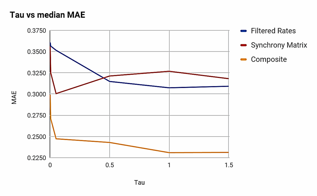
5.4. Role of memory

As expected, the value of Tau had a deep impact on performance. The difference between best and worst performance across a few sample points corresponding to Tau values ranging from 0 to 1.5 can be as high à 22.81% in the cast of the composite-state representations (see Table 4). It is also clear from Figure 10 that the relationship between memory and performance is nonlinear and dependent on the type of liquid state representation.

Table 4: Impact of memory on performance

5.5. Separation measures

We expect a negative correlation between the Separation measure and classification error. The magnitude of this correlation is an indication of how good a predictor of performance SP is. As shown in Figure 11, FDR performs best among the “classical” SP measures (Centroids, Ranks, Van Rossum distance, Gaussian distance). On the other hand, the newly introduced separation measures based on spike metrics seem to correlate even more with the classification performance of LSMs. The measures based on spike synchronization, ISI-distance (and its adaptive variant), adaptive rate-independent spike distance, and Schreiber correlation all correlate below the -0.5 mark.

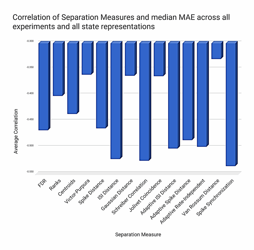
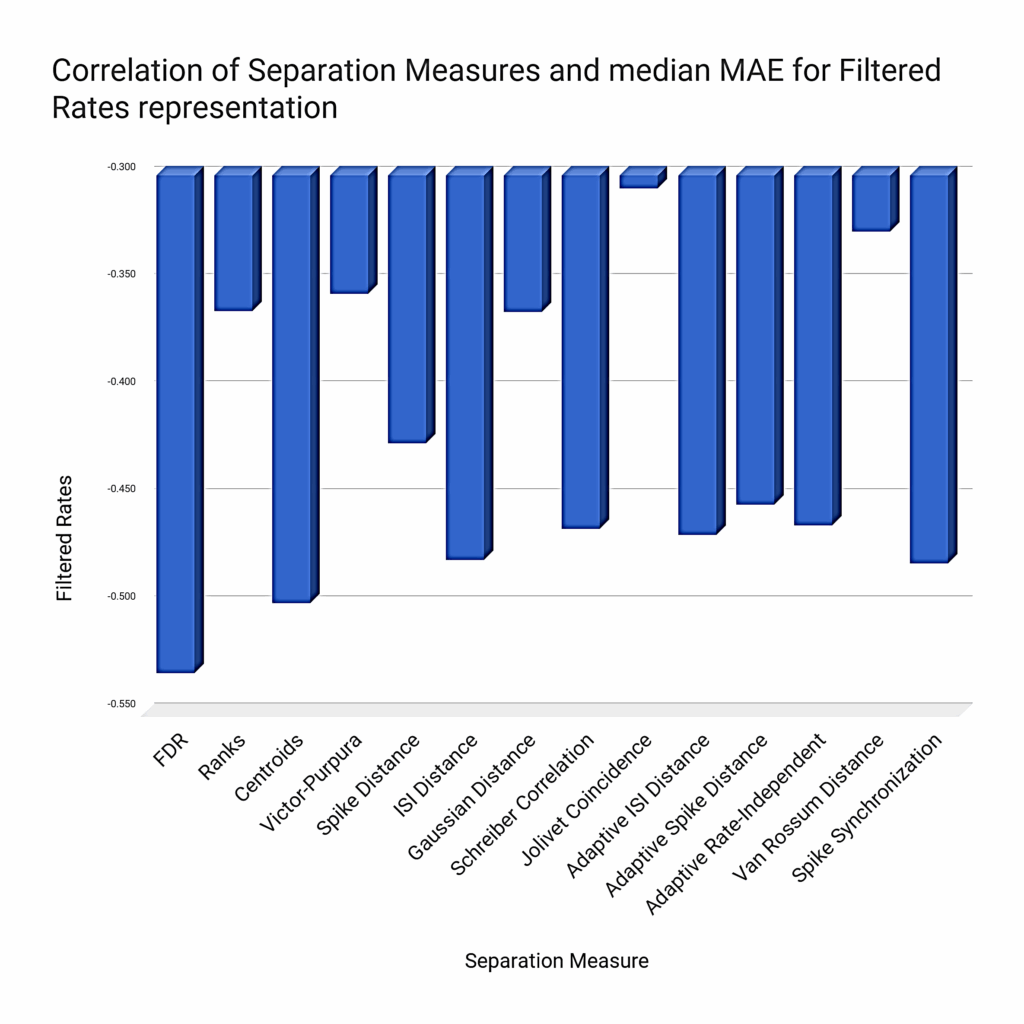
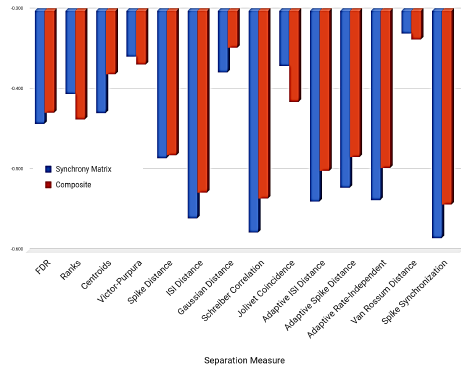
However, this synthetic chart shown in Figure 11 hides the local discrepancies between the different measures, since some of them perform significantly better in certain situations. For instance, Figure 12 shows that FDR correlates generally better with rate-based representations, but Figure 13 shows the opposite for synchrony-based representations (either using a synchrony matrix or a composite-state representation).

6. Discussion and future research

At the core of each LSM study lies a neuron/synapse simulator for validation. It is not only a model of computation, but also a simplified model of the cortical columns found in real-life neural systems. This biological inspiration suggests that neuroscientific discoveries regarding the understanding of the “neural code” may also enhance the computational model. We discuss below our findings on rate and temporal coding, the role of SP as a performance predictor, and the influence of sampling and memory on performance before ending this paper with a short review of the results of other comparable studies and concluding.

6.1. Rate and temporal decoding

The temporal decoding of liquid states can easily match the levels of LSM classification performance reached by rate-decoding approaches, while composite state feature vectors go beyond: they allowed to raise the overall performance without increasing the LSM dimensionality, even in the context of highly noisy inputs. These findings point to the critical role of phase information and temporal decoding in LSM classification, encouraging more research to explore temporal coding and decoding schemes. For instance, more encoding strategies based on phase information or absolute spike timings ought to be investigated (see [60] for inspiration), as well as more advanced spike rate estimation mechanisms (several of them are presented in [61]). With regards to performance, this study also found that the liquid state sampling frequency (in the light of its relationship to memory capabilities) and the topology of connections are critical factors, and they could thus become targets of optimization for peak performance. But, as the next subsection shows, the currently proposed measures of SP do not correlate well enough with LSM classification performance.

On the negative side, one major limitation of the synchrony matrix representation of liquid states is that the matrix grows with liquid size, with a quadratic impact on the synchrony vector size (equation 5). For example, for a 2x2x2 liquid, the number of elements of the feature vector is 28 as already mentioned, and for a 4x4x4 liquid, this number reaches 2080 (from equation 5 with N=64). Large feature vectors tend to promote overfitting: for instance, the linear regression that we use as a classifier quickly becomes overwhelmed with them. Several ideas can be put forward to cope with large-size liquids and reduce the dimensionality of the feature vectors. They include:

• Principal Component Analysis of the synchrony matrices for dimensionality reduction.
• Hierarchical construction of liquids: connecting a large liquid to gradually smaller ones until a suitably small liquid is found.
• Stochastic sampling of pairs of neurons in the liquid and subsequent reconstruction of the synchrony and rate information (also suggested in [5]).
• Temporal filtering and fuzzification: creating aggregate spike trains from liquid subregions (for example, we filter 2x2x2 regions in a 6x6x6 liquid to create a 3x3x3 “aggregate” liquid) and applying a form of temporal filtering, replacing multiple spikes emitted within a certain “fuzzy” timeframe by a single one at the mean of the that interval.

However, although temporal decoding may be a promising technique, it does not solve the performance variability across liquids. One way to address this problem is to determine performance predictors and engineer more efficient liquids.

6.2. Performance predictors and liquid optimization

The differences between “classical” SP and synchrony-based measures seem to highlight some complementarity between the two approaches. On average, our measure of SP roughly explained 50% of the performance of an artificial classification experiment (the absolute amount of correlation between SP and generalization error was, at best, slightly over 0.5). So, a question remains: what is missing from SP measures that could explain the missing 50%? Two very broad hypotheses can be put forward:

a)    Other performance predictors should be used instead of or in conjunction with SP;

b)    Our evaluation of  SP is incomplete or deficient: some crucial information may not be captured by statistical methods, linear algebra or spike distance metrics.

While more SP measures (Bray-Curtis [62] and other vector distances [63], etc.) should be tested, we think that a custom, composite SP measure built out of rate and synchrony information should also  be investigated. Indeed, synchrony-based or hybrid measures tend to correlate better with synchrony-based state representations while statistical measures perform better with rate-based representations. These results seem to hint that the ideal separation measure could be a hybrid of FDR and synchrony metrics, exploiting the idea that phase and rate information are complementary representations of the same spiking activity.

6.3. Memory and state sampling frequency

Our results also show that the memory capacity of a liquid has an impact on classification performance, particularly when using composite-state representations (over 22% gap between best and worst performance, significantly higher than for rate-based or synchrony-only representations). Determining the optimal memory parameters and sampling frequency to extract enough information while preserving temporal resolution and avoiding pathological memory conditions deserves attention. The standard approach to divide the time axis into same-duration bins can create two problems: a) empty states, b) window boundary issues, especially for synchrony calculation (spikes fired just before or after the time window boundaries are not accounted for).

We observed a significant degradation of performance when the state sampling frequency was increased (illustrated in Figure 7), attributed to the decline of the information content of each sample and the increased time resolution. The reduction of the width of the sampling time window has two consequences:

1. a) More state samples required to cover the entire simulation , with the compounded sampling error most likely increased (i.e., the probability of missing relevant spikes at the boundaries of each time window).
2. b) Lower average number of spikes that can be captured in each sample, which in turn augments the impact of missed spikes on the total count of spike firings.

These two combined effects can lead to less reliable feature vectors. Low spiking activity also happens during network “warm up”, as discussed in [6] and [17].  A solution to these problems may be to use interleaved sampling with window smoothing as done in automatic voice recognition systems.

6.4. Related work on LSM performance

Several authors have explored the question of the classification performance of the LSM model and highlighted its strengths and limitations in various contexts, but there seems to be a relative dearth of results comparable to ours, as methodologies and data vary significantly across studies. It is also worth noting that we have deliberately left out research on readout performance, although works such as [64] show that this crucial element of the LSM model can also be improved.

Putting aside the previous caveats, the conclusions we draw from this work are very much in line with those of the seminal work of Maass and al. [23] who validated the role of SP in LSM performance using a globally comparable method. In our work, we looked at this problem from the angle of liquid state representations, but numerous studies have focused on other aspects and suggested techniques to increase both the separability and the generalization properties of an LSM. The list includes:

• Optimizing the connection topology and the synaptic weights ([65], [19], [13], [17], [18]);
• Careful selection or mixtures of neuron types ([23], [66], [16], [1]);
• Addition of parallel columns [23];
• Construction of hierarchical liquids [16];
• Correct choice or composition of liquid state representations [10];
• Selection of the right memory parameters [3];
• Usage of ensemble techniques [5].

In addition, the problem of quantifying SP remains open. In [62] and [37], the authors indicate that their own custom measure of SP outperforms those based on either the ubiquitous Gaussian distance or the Van Rossum metric, but they did not provide correlation results with actual performance. Similarly, compelling evidence of a strong correlation between classification performance and SP is reported in [14]. The measures proposed by [3], [18] and [13] correlate to levels up to 0.79, 0.68 and 0.86 respectively, whereas our own results show an average correlation of only slightly above the 0.5 mark, a discrepancy than can be explained by the differences in the methodologies and validation contexts.

7. Conclusion

In this paper, we have shown through simulation experiments that the temporal decoding of spike trains by evaluation of the synchrony between pairs of neurons in the liquid can improve the LSM performance for classification tasks. We have also shown that the Separation Property, a fundamental characteristic of LSMs, can reliably be measured by spike metrics.

While there is a strong consensus in the research community that the classification performance of the LSM model can be raised, no definitive solution has yet emerged. We believe that more research is needed to improve the aforementioned approaches and/or combine their strengths to improve the LSM core performance in classifying time-varying input data. We also think that the results presented here should be tested and validated on a larger scale. Moreover, if the temporal decoding of liquid states improves classification performance, its efficiency in a less artificial context remains to validate.

1. W. Maass, “Liquid State Machines: Motivation, Theory, and Applications,” World Scientific Review, Vol. March 25/2010, doi: 10.1142/9781848162778_0008
2. D. Verstraeten, B. Schrauwen, B., D. Stroobandt, “Isolated word recognition with the liquid state machine: a case study,” Proc. 13th European Symposium on Artificial Neural Nets (ESANN), vol. 95(6), pp. 435–440, 2005.
3. E. Goodman, E., Ventura, D. “ Spatiotemporal pattern recognition via liquid state machines,” International Joint Conference on Neural Networks (IJCNN), pp. 3848–3853, 2006.
4. W. Maass, T. Natschlager, H. Markram, “Fading memory and kernel properties of generic cortical microcircuit models,”Journal of Physiology (Paris), vol. 98, pp. 315–330, 2004.
5. J. De Gruijl, M. Wiering, “Musical Instrument Classification using Democratic Liquid State,” Proc. 15th Belgian-Dutch Conference on Machine Learning, 2006.
6. L. Pape, R. Jornt, J. De Gruijl, M. Wiering, “Democratic Liquid State Machines for Music Recognition”, Speech, Audio, Image and Biomedical Signal Processing using Neural Networks. Volume 83b, Berlin, 2008.
7. J. Hertzberg, H. Jager, F. Schonherr. F., “Learning to ground fact symbols in behavior-based robot,” Proc. 15th European Conference on Artificial Intelligence., pp. 708–712, Amsterdam, 2002.
8. H. Burgsteiner, M. Kroll, A. Leopold, G., Steinbauer, “Movement prediction from real-world images using a liquid state machine,” Appl. Intell. vol. 27 (2), pp. 99–109, 2007.
9. H. Ju, J. Xu, A. VanDongen, A. “Classification of Musical Styles Using Liquid State Machines,” Proc. International Joint Conference on Neural Networks s (IJCNN), 2010, doi: 10.1109/IJCNN.2010.5596470.
10. F. Rhéaume, D. Grenier, E. Bosse, “Multistate combination approaches for liquid state machine in supervised spatiotemporal pattern classification,” Neurocomputing, vol. 74, pp. 2842–2851, 2011.
11. M. Aoun, M. Boukadoum, “Chaotic Liquid State Machine,” International Journal of Cognitive Informatics and Natural Intelligence, vol. 9(4), 1-20, October-December 2015
12. J. Huang, H. Fang, Y. Wang, “ Directional classification of cortical signals using a liquid state machine,” Proc. 17th World Congress of The International Federation of Automatic Control, Seoul, Korea, July 6-11, 2008.
13. E. Hourdakis, P. Trahanias , “Use of the separation property to derive Liquid State Machines with enhanced classification performance,” Neurocomputing, vol. 107, pp40–48, 2013.
14. R. Legenstein, W. Maass, “Edge of chaos and prediction of computational performance for neural circuit models, Neural Networks, vol 20(3), pp. 323–334, 2007.
15. D. Norton, D. Ventura, “Preparing More Effective Liquid State Machines Using Hebbian Learning,” Proc. International Joint Conference on Neural Networks (IJCNN), 2006.
16. J. Matser, “ Structured liquids in liquid state machines,” (Master Thesis, Utrecht University, 2010).
17. S. Kok, “Liquid State Machine Optimization,” (Master Thesis, Utrecht University, 2007).
18. D. Norton, D. Ventura, “Improving the performance of liquid state machines through iterative refinement of the reservoir,” Neurocomputing, vol. 73, pp. 2893–2904, 2010.
19. J. Huang, Y. Wang, J. Huang, “The Separation Property Enhancement of Liquid State Machine by Particle Swarm Optimization,” International Symposium on Neural Networks (ISNN 2009: Advances in Neural Networks), pp 67-76, 2009.
20. A. Kasinski, F. Ponulak, “Comparison of supervised learning methods for spike time coding in spiking neural networks,”.Int. J. Appl. Math. Comput. Sci., vol. 16(1), pp. 101–113, 2006.
21. T. Kreuz, T. (2001). Measures of spike train synchrony, Scholarpedia, vol. 6(10):11934, 2001.
22. http://www.scholarpedia.org/article/Measures_of_spike_train_synchrony
23. W. Maass, T. Natschlager, H. Markram, H. “Real-time computing without stable states: A new framework for neural computation based on perturbations,” Neural Computation, vol. 14(11), pp. 2531–2560, 2002.
24. D. Buonomano, W. Maass, “State-dependent computations: Spatiotemporal processing in cortical networks,” Nature Reviews in Neuroscience, vol. 10, no. 2, pp. 113–125, 2009.
25. J. Mayor, W. Gerstner, “ Transient information flow in a network of excitatory and inhibitory model neurons: role of noise and signal autocorrelation,” Journal of Physiology (Paris), vol. 98, pp. 417–428, 2004.
26. CSIM user manual: http://www.lsm.tugraz.at/download/csim-1.1-usermanual.pdf
27. R. Legenstein, H. Markram, W. Maass, “Input prediction and autonomous movement analysis in recurrent circuits of spiking neurons,” Reviews in the Neurosciences (Special Issue on Neuroinformatics of Neural and Artificial Computation), vol. 14, no. 1-2, pp. 5–19, 2003
28. S. Hausler, H. Markram, W. Maass, “Perspectives of the high-dimensional dynamics of neural microcircuits from the point of view of low-dimensional readouts”. Complexity, vol. 8(4), pp. 39–50, 2003.
29. A. Oliveri, R. Rizzo, A. Chella, “An application of spike-timing-dependent plasticity to readout circuit for liquid state machine,” IEEE International Joint Conference on Neural Networks, pp. 1441–1445, 2007.
30. H. Ju et al., “Effects of synaptic connectivity on liquid state machine performance,” Neural Networks, vol. 38, pp. 39–51, 2013.
31. R. Brette, “Philosophy of the Spike: Rate-Based vs. Spike-Based Theories of the Brain,”. Front. Syst. Neurosci. 2015, doi: 10.3389/fnsys.2015.00151
32. B. Meftah et al., “Image Processing with Spiking Neuron Networks,” Artif. Intell., Evol. Comput. and Metaheuristics, SCI 427, 525–544, 2012.
33. J. D. Victor, “Spike train metrics,” Current Opinion in Neurobiology, vol. 15, pp. 585–592, 2005.
34. T. Kreuz, “Measures of spike train synchrony,“ Scholarpedia, vol. 6(10), pp. 11934, 2001.
35. W. Gerstner et al., Neuronal Dynamics: From single neurons to networks and models of cognition, Cambridge University Press, 2014, http://neuronaldynamics.epfl.ch/online/Ch7.S6.html.
36. G. B. Stanley, “Reading and writing the neural code,” Nature Neuroscience, vol. 16, pp. 259–263, 2013, doi:10.1038/nn.3330
37. K. P. Dockendorf et al., “Liquid state machines and cultured cortical networks: the separation property,” Biosystems, vol. 95(2), pp. 90–97, 2009.
38. M. C. W. Van Rossum, “A novel spike distance,” Neural Comput., vol. 13, pp. 751–763, 2001.
39. J. D. Victor, K. P. Purpura K.P., “Spike Metrics,” In: Analysis of Parallel Spike Trains. Ed. Stefan Rotter and Sonja Gruen. Springer, pp. 129-156, 2010. http://www-users.med.cornell.edu/~jdvicto/pdfs/vipu10.pdf.
40. E. Satuvurori et al., “ Measures of spike train synchrony for data with multiple time scales,” J Neurosci. Meth, vol. 287, pp. 25-38, 2017
41. T. Kreuz et al., “Measuring spike train synchrony,” J Neurosci Meth., vol. 165, pp. 151–161, 2007.
42. T. Kreuz et al., “Measuring synchronization in coupled model systems: a comparison of different approaches,” Phys D., vol. 225, pp. 29–42, 2007.
43. T. Kreuz et al., “Measuring multiple spike train synchrony,” J. Neurosci Meth., vol. 183, pp. 287–299, 2009.
44. T. Kreuz, D. Chicharro, M. Greschner, R. G. Andrzejak, “Time-resolved and time-scale adaptive measures of spike train synchrony,” J. Neurosci Meth., vol. 195, pp. 92–106, 2011.
45. T. Kreuz et al., “Monitoring spike train synchrony,” J. Neurophysiol., vol. 109, pp. 1457-72, 2013.
46. http://www.scholarpedia.org/article/SPIKE-distance
47. J. D. Victor, K. P. Purpura, ”Nature and precision of temporal coding in visual cortex: a metric-space analysis,” J. Neurophysiol., vol. 76, pp. 1310–1326, 1996.
48. J. D. Victor, K. P. Purpura, ”Metric-space analysis of spike trains: theory, algorithms and application, Network, vol. 8, pp. 127–164, 1997.
49. S. Schreiber et al., “A new correlation-based measure of spike timing reliability,” Neurocomputing, vol. 52, pp. 925–931, 2003.
50. J. D. Hunter, G. Milton, G., “Amplitude and frequency dependence of spike timing: implications for dynamic regulation,” J. Neurophysiol., vol. 90, pp. 387‐394, 2003.
51. R. Quian Quiroga, T. Kreuz, P. Grassberger, “Event synchronization: a simple and fast method to measure synchronicity and time delay patterns,” Phys Rev E Stat Nonlin Soft Matter Phys, vol. 66:041904, 2002, doi: 10.1103/PhysRevE.66.041904.
52. T. Kreuz, M. Mulansky, N. Bozanic, “SPIKY: A graphical user interface for monitoring spike train synchrony,” J Neurophysiol., vol 113, pp. 3432, 2015.
53. R. Jolivet et al., “A benchmark test for a quantitative assessment of simple neuron models,” J Neurosci Meth., vol 169, pp. 417–424, 2008.
54. http://www.lsm.tugraz.at/download/circuit-tool-1.1-manual.pdf
55. T. Natschlager, W. Maass, H. Markram. Chapter 9, Computer Models and Analysis Tools for Neural Microcircuits, http://www.lsm.tugraz.at/papers/lsm-koetter-chapter-144.pdf
56. http://www.lsm.tugraz.at/download/csim-1.1-usermanual.pdf
57. H. Markram, Y. Wang, M. Tsodyks, “ Differential Signaling via the Same Axon of Neocortical Pyramidal Neurons,” Proc Natl Acad Sci U S A., 1998, doi: 10.1073/pnas.95.9.5323..
58. CSIM: A neural Circuit SIMulator, http://www.lsm.tugraz.at/csim/
59. R. Brette et al., “Simulation of networks of spiking neurons: A review of tools and strategies,” J. Comput Neurosci., vol. 23(3), pp. 349-98, 2007, doi 10.1007/s10827-007-0038-6
60. B. Gardner, I. Sporea, A. Gruning, “Encoding Spike Patterns in Multilayer Spiking Neural Networks,” arxiv.org/abs/1503.09129v1, 2015.
61. S. Shinomoto, S. Grun, S. Rotter, S. (2010). Chapter 2, Estimating the Firing Rate. Analysis of Parallel Spike Trains, in S. Grün, S. Rotter (eds.), Analysis of Parallel Spike Trains, Springer Series in Computational Neuroscience 7, 2010, doi 10.1007/978-1-4419-5675-0_2
62. G. M. Wojcik, M. Wazny, “ Bray-Curtis Metrics as Measure of Liquid State Machine Separation Ability in Function of Connections Density,” Procedia Computer Science, Vol. 51, pp. 2938–2942, Proc. International Conference on Computational Science (ICCS), 2015.
63. M. Loginov, “Beyond decoding: representational similarity, analysis on fMRI data,” (Master’s Thesis, University of Tartu, 2015).
64. S. Roy, A., Banerjee, A. Basu, “Liquid State Machine with Dendritically Enhanced Readout for Low-power, Neuromorphic VLSI Implementations,” IEEE Trans. Biomedical Circuits and Systems, vol. 8(5), pp. 681-695, 2014. doi: 10.1109/TBCAS.2014.2362969
65. H. Hazan, L. M. Manevitz “Topological constraints and robustness in liquid state machines,” Expert Systems with Applications, vol. 39, pp. 1597–1606, 2012.
66. B. J. Grzyb, E. Chinellato, G. M. Wojcik, W. A. Kaminski, W.A., “Which model to use for the Liquid State Machine?” Proc. International Joint Conference on Neural Networks (IJCNN), pp. 1018-1024, 2009, doi: 10.1109/IJCNN.2009.5178822.

Citations by Dimensions

Citations by PlumX

Crossref Citations

1. Nicolas Pajot, Mounir Boukadoum, “Fire Type Classification in the USA Using Supervised Machine Learning Techniques”, Journal of Engineering Research and Sciences, vol. 4, no. 6, pp. 1–8, 2025. doi: 10.55708/js0406001
2. Nicolas Pajot, Mounir Boukadoum, “Water Potability Prediction Using Neural Networks”, Journal of Engineering Research and Sciences, vol. 4, no. 5, pp. 1–9, 2025. doi: 10.55708/js0405001
3. Nicolas Pajot, Mounir Boukadoum, “Fuzzy-Based Approach for Classifying Road Traffic Conditions: A Case Study on the Padua-Venice Motorway”, Journal of Engineering Research and Sciences, vol. 3, no. 11, pp. 31–40, 2024. doi: 10.55708/js0311003
4. Nicolas Pajot, Mounir Boukadoum, “MCNN+: Gemstone Image Classification Algorithm with Deep Multi-feature Fusion CNNs”, Journal of Engineering Research and Sciences, vol. 3, no. 8, pp. 15–20, 2024. doi: 10.55708/js0308002
5. Nicolas Pajot, Mounir Boukadoum, “Quantum Machine Learning on Remote Sensing Data Classification”, Journal of Engineering Research and Sciences, vol. 2, no. 12, pp. 23–33, 2023. doi: 10.55708/js0212004